Wave-Wave Interactions: Fourier Analysis: Non-Periodic Functions

  If a function S(t) is not periodic, the Fourier components that make up that function no longer need to repeat after some characteristic time. As a results, we can have a continuous range of frequencies that make up the function S(t) and the discrete Fourier sum that we used for periodic functions on the previous page now becomes a continuous integral. The Fourier components now have a continuous range of frequencies ω=2π f, so we can no longer use the discrete index n to label each component's amplitude, frequency, and phase as we did for periodic functions in the last page. Now the amplitudes and phases are functions of the continuous frequency variable ω.

  Before going to a strictly continuous range of frequency components, let's begin with a periodic function S(t) with a period τ with discrete frequencies. Imagine that the function S(t) is made up of many arbitrarily closely spaced frequency components, each separated by dω. One can reach the continuous range of frequency components by letting the period τ aproach infinity. Since the Fourier components must repeat after this long period and their frequencies are given by ω_n=n×2 π/τ, the spacing between neighboring frequencies is dω=2π/τ and goes to zero as τ goes to infinity.

  Let's take a look at S(t) at one moment in time when t=t_c. Each frequency is now given by ω_n= n dω. As dω approaches zero, the series of amplitudes A_n (bars in the graph below) and phases φ_n become smooth functions A(ω) and φ(ω), respectively. You will see in a moment why we divided A(ω) by the constant dω in the graph below.

  In the equation below we show the discrete Fourier sum for S(t) before letting τ approach infinity.

  If we multiply the right hand side of the equation above by dω/dω and let dω approach zero (which occurs when τ approaches infinity), the sum becomes an integral, as shown below:

where A'(ω)=A(ω)/dω can be thought of as an amplitude density, i.e, the amount of amplitude within the frequency range between ω and ω+dω. The equation above holds for any time t, so we can replace t_c with the variable t. Therefore, we see that if we have a continuous distribution of frequency components with amplitudes given by A(ω), S(t) at any given time is simply proportional to the area under the curve A(ω)sin(ωt+ φ(ω)) at that same time.

  The orthogonality relations that we used for periodic functions still hold, except now ω and ω_ref are continuous variables:

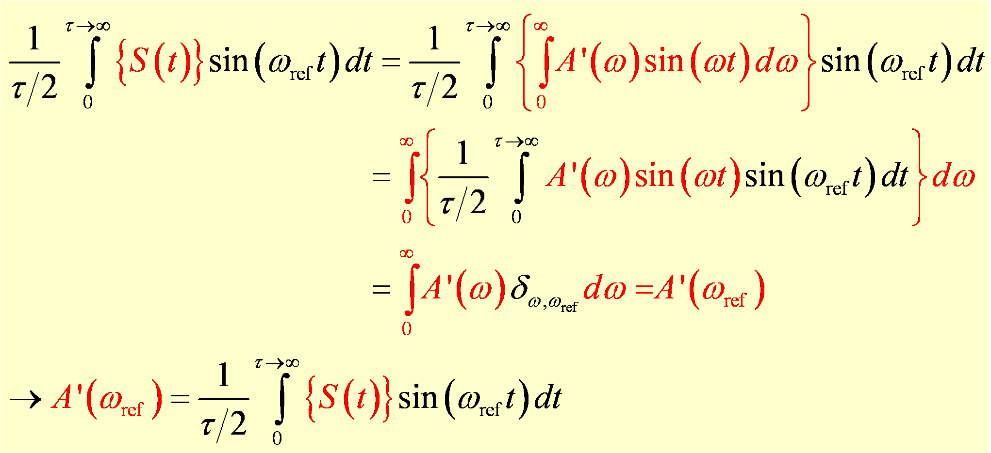
Just as with periodic functions, we can use the orthogonality of Fourier components to determine the amplitudes for the continuous set of components that contribute to a non-periodic function. In this case however, instead of getting a series of discrete amplitudes A_n, we obtain a continuous amplitude function A'(ω). In order to determine the amplitude of the component at a reference frequency ω_ref contained in S(t), we multiply S(t) by the sin( ω_reft) and integrate the product over time. As with the case for periodic functions, the components in S(t) that are not at frequency ω_ref will integrate to zero. Note that in this case, one integrates over time before integrating over frequency. The time integration produces a Kronecker delta function which picks out the value of A' at ω_ref when integrating over all positive frequencies.

  Here is a Fourier analysis java applet that lets you find sinusoidal wave components in a function. Here we allow a more continuous spectrum of components, where the reference components are not harmonics of a common lowest frequency, e.g., do not go to zero at right side of the graph as S(t) does. Although the signal function in this case is periodic, we can use continuous Fourier analysis on any function within a given range.

• Press "Load Curve" button to load the Signal function.
• Set the "Integration Time" slider to a lower value ~8. This represents the time over which the (Signal)x(Reference) product is averaged.
• Slowly move "Reference Frequency" slider over its full range to select different reference functions.
• Observe how the Signal*Reference product averages to zero unless the Reference frequency is the same as one of the components in the Signal. Note that if the reference frequency is close but not exactly the same as one of the frequencies in the Signal, the average is not exactly zero since the time over which one averages may not be long enough to get the negative contributions to cancel the positive contributions to the average. If the frequencies are close, the product will tend to be positive until one eventually falls behind the other. This is similar to what happens when two waves with nearly the same frequency are ADDED (beating), but note that we are actually MULTIPLYING waves here!
• Check the alignement of dips and peaks in the Signal and Reference panels; Check the (Signal)x(Reference) product panels; Check the Product Average window, which shows the integrated average of the (Signal)x(Reference) product.
• Set the Reference frequency to a position where the Product Average is a maximum and move the phase slider to change the phase of the Reference function with respect to the Signal. What happens when they are 90 degrees out of phase? What happens when they are 180 degrees out of phase?
• Increase the integration time to a higher value closer to 16 and move the Reference frequency slider through its full range again. Is there any difference? Why?
• For longer integration times, notice how much sharper the peaks are in the (|Product Average|) window. If we are able to look at waves over very long times we are better able to distinguish two waves that have slightly different frequencies!This is the basis for Heisenberg's Frequency-Time (or Energy-Time) uncertainty principle!
• Notice the higher frequency oscilations in the spectrum shown in the Product Average panel. These occur because the functions are sharply cut off at the ends of the time integration window. As the reference frequency changes, the contributions from these cut off ends oscillates, causing the average to also oscillate. Another way to think of it is that cutting the data to a finite length artificially introduces another frequency/period that corresponds to the width of the time averaging window. The oscillatory artifacts can be reduced by forcing Reference*Signal to smoothly go to zero at the boundaries of the time-averaging window. This is called apodization and is used to clean up results when Fourier analysis is applied to finite length data, such as audio signal processing or image processing, i.e., photos also have edges! Select the "Apodize Curve" check box to smooth the ends of the data. If one is concerned about the quantitative results, one should rescale the product average when the data are apodized since we are reducing the values of the product at the ends of the range, but since we wish only to show the qualitative effects of apodization, we have not rescaled the "Product Average" results.